If you’ve ever wanted to make your Google Sheets feel more interactive and user-friendly, adding a date picker is a simple and powerful way to do it. Whether you’re managing a project timeline, tracking tasks, or creating a form, letting users choose from a calendar dropdown instead of typing dates manually can save time and reduce errors.
In this tutorial, we’ll show you exactly how to add a calendar date picker to any cell (or column) in Google Sheets using the built-in Data Validation feature.
✅ What You’ll Learn
- How to add a calendar popup to cells in Google Sheets
- How to apply it to a column
- How to remove or adjust the setting later
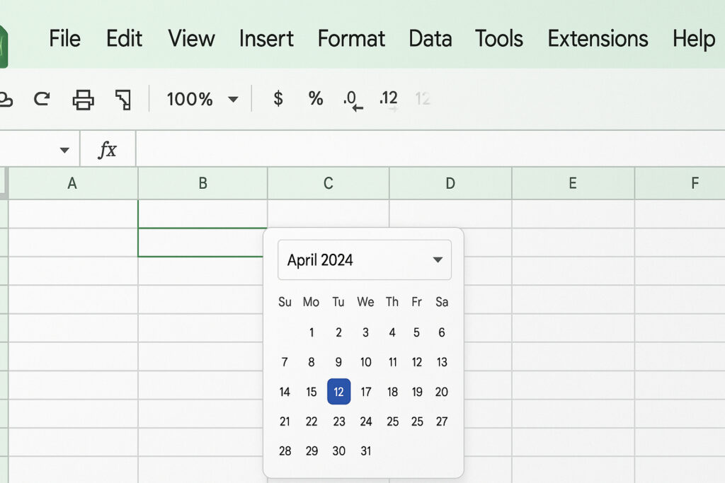
🖼️ Date Picker Example
🛠️ Step-by-Step: How To Add a Date Picker in Google Sheets
- Select the Cell(s): Click on the cell or range of cells where you want to enable the calendar dropdown.
- Open Data Validation: Go to
Data > Data validation. - Set the Criteria to Date: Choose “Date” as the criteria.
- Enable the Calendar Dropdown: Check “Show dropdown calendar.”
- Click Done: Now click the cell again — a calendar popup should appear.
🔄 Bonus Tip: Apply It to a Whole Column
Apply the data validation to A2:A to enable the picker for all new entries.
❌ Removing the Date Picker
To remove it, select the cell(s), go to Data > Data validation, and click Remove validation.
📌 Final Thoughts
Adding a date picker is an easy win to improve user experience in any spreadsheet. It makes data entry faster, more accurate, and way more polished.
🎥 Watch the Full Video: